みなさんこんにちは!このブログでは主に
の4つのトピックについて発信しています。
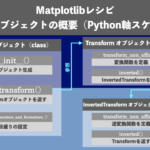
今回はPythonデータ解析です!Matplotlib、軸のスケールシリーズ第4回!Logスケールを例に、Scale class、Transform class、InvertedTransform classの概要を解説します!LogScale、LogTransform、InvetedLogTransformという3つのClassの使い方をセットで理解しておくことで、Pythonで作図する際に軸のスケールを対数にしたり、変換・逆変換関数を簡単に呼び出せるようになります。
この記事を読めば、軸のスケールの設定だけでなく、変換関数や逆変換関数を呼び出して使う方法を知ることができます!ぜひ最後までご覧ください。
この記事はこんな人のお悩み解決に役立ちます!
- Pythonの作図で軸のスケールを変えたいけどどうやる?
- 変換関数や逆変換関数を自在に呼び出すには?
Abstract | Logスケールと変換関数の関係をマスター
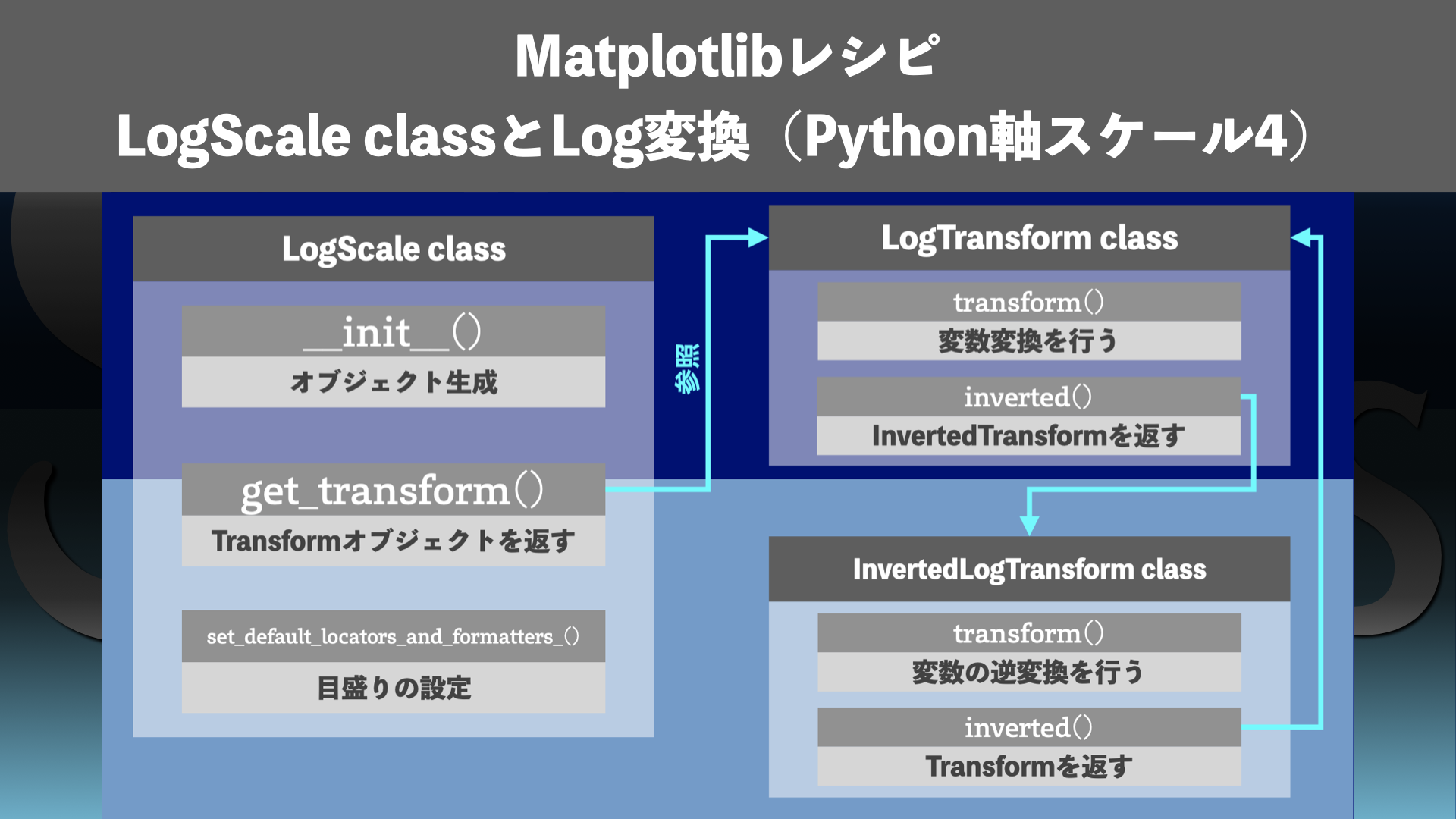
MatplotlibでLogスケールの描画を行う場合、スケール設定に用いるLogScale classとLog変換を行う関数やその逆変換を行う関数と関係を頭に入れておくと、描画の際に変換関数や逆変換関数を自在に呼び出せるようになります。
Log変換を行う変換関数はLogTransform class、逆変換の関数はInvertedLogTransform classとして定義されています。それぞれのクラスのtransform()メソッドを用いることで、変数変換や変数の逆変換を行うことができます。
LogTransform classはLogScale classからget_transform()メソッドで呼び出すことができ、InvertedLogTransform classはLogTransform classからinverted()メソッドで呼び出すことができます。このような相互関係を知っておくと、プロットと変数変換を組み合わせた処理を簡単に実装することができます。
Background | PythonのスケールとScaleオブジェクト
散布図やヒストグラム、その他さまざまな図を作る際、軸のスケールを適切に設定する必要があります。Pythonの作図ライブラリMatplotlibでは、デフォルトの線形スケール以外に様々スケールでプロットすることができます。プロットしたいデータの分布に合わせて適切なスケールを選ぶことが必要です。
本シリーズの過去記事
- Matplotlib | Python作図での軸のスケール設定の必要性(Python軸スケール 1. 知識編)
- Matplotlib | 予め用意された7種類のスケール(Python軸スケール2)
- Matplotlib | Scale Classの概要(Python軸スケール3)
では、線形スケールでは図を綺麗に表示できない例や、Matplotlibに予め定義されたスケールを使ってプロットする方法、Matplotlibのスケールを制御するScale Classについて解説してきました。
今回の記事では前回取り扱ったScale ClassのうちLogスケールについて扱います。LogScale Class、LogTransform Class、InvertedLogTransform Classについて解説します。より詳しく知りたい方はMatplotlibのドキュメントページは(matplotlib.scale)もご覧ください。
Method | LogScale Classの使い方
Matplotlibで用意されている7つのスケールのうち、Logスケールについての3つのClass
- LogScale Class
- LogTransform Class
- InvertedLogTransform Class
の動作を確認していきます。
ここからはJupyter Notebookを使ってコードの書き方も記載するので、一緒にコードを動かしながら読んでみてください!ここで用いた関数を通常のPythonソースコードにコピーして使ったり、Pythonのファイルにまとめてimportして使ってもOKです!
Resultの章にJupyter Notebookでの実装例を掲載するので、そちらを参照していただいても構いません。この章では、簡単な解説とともにソースコードを一つずつ提示します。解説が不要な方はResultの章に飛んでいただき、Jupyter Notebookでの実装例を参考にする方が早いかもしれません。
各種事前準備
まずはJupyter Notebookのファイルを開きましょう。Jupyter Notebookの使い方については過去記事「python入門講座|pythonを使ってみよう2(Jupyter Notebookを使う方法)[第5回]」もご覧ください!
ライブラリのインポート
Jupyter Notebookを開いたらライブラリをインポートします。今回はNumPyとMatplotlib関連のライブラリをいくつかインポートしておきます。以下を実行します。
import numpy as np
import matplotlib as mpl
import matplotlib.pyplot as plt
import matplotlib.gridspec as gridspec
Matplotlibのバージョン確認
Matplotlibのバージョンも確認しておきます。今回に関してはバージョンを気にする必要はありませんが、3.8以降にしておくと過去記事「Matplotlib | 予め用意された7種類のスケール(Python軸スケール2)」で紹介した7つのスケールを全て使うことができます。以下を実行します。
mpl._version.version実行結果は以下のように表示されます。
'3.8.0'
予め用意されたスケールを確認
Matplotlibで予め用意されたスケールを確認しておきます。以下を実行します。
mpl.scale.get_scale_names()実行結果は以下のように表示されます。ここに’log’があれば問題ありません。
['asinh', 'function', 'functionlog', 'linear', 'log', 'logit', 'symlog']
文字列”log”を使ってLogスケールを描画する方法
y軸をLogスケールにしてplotする例を扱います。まずは一番シンプルな方法でy軸をLogスケールにする方法です。以下を実行してみてください。
# set x and y
x = np.random.normal(size=1000)
y = 10**(x+np.random.normal(size=np.shape(x)))
# plot with log-scale y
fig = plt.figure(figsize=[8,4])
gs = gridspec.GridSpec(1, 2, wspace=0.3)
axs = {}
# linear scale
i = 0
axs[i] = plt.subplot(gs[i])
axs[i].set_title('Example in linear scale')
axs[i].set_xlabel('x')
axs[i].set_ylabel('y')
axs[i].scatter(x, y)
# log scale
i = 1
axs[i] = plt.subplot(gs[i])
axs[i].set_title('Example in log scale')
axs[i].set_xlabel('x')
axs[i].set_ylabel('y')
axs[i].set_yscale('log')
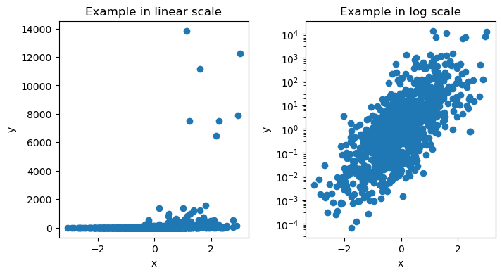
axs[i].scatter(x, y)実行すると以下の図が表示されます。乱数が入っているので、散布図の点の位置は実行するたびに変わります。
なお、上記のコードセルの中で、
axs[i].set_yscale('log')という箇所でy軸をLogスケールに変更しています。x軸をLogにしたい場合には
axs[i].set_xscale('log')とします。
LogScale Classを使ってLogスケールで描画する方法
`matplotlib.scale`には`xxxScale`というclassが用意されています(xxxにはLog, Logit, SymmetricalLogなどが入ります)。詳細は過去記事「Matplotlib | 予め用意された7種類のスケール(Python軸スケール2)」をご覧ください。前述のMatplotlibでスケールを設定する描画例のような”log”といった文字列ではなく、`xxxScale` classのオブジェクトを`ax.set_yscale()`などに渡すことで、y軸などのスケールを変更することができます。
ここでは`x`と`y`は先程の例と同じにし、Logスケールの設定を`LogScale` classを使って行います。`mpl.scale.LogScale(axs[i])`のように、matplotlib.axisオブジェクトを引数として与えて`LogScale` classのオブジェクトを作って`set_x/yscale()`に渡します。以下を実行してください。
# plot with log-scale y
fig = plt.figure(figsize=[8,4])
gs = gridspec.GridSpec(1, 2, wspace=0.3)
axs = {}

# linear scale
i = 0
axs[i] = plt.subplot(gs[i])
axs[i].set_title('Example in linear scale')
axs[i].set_xlabel('x')
axs[i].set_ylabel('y')
axs[i].scatter(x, y)

# log scale
i = 1
axs[i] = plt.subplot(gs[i])
axs[i].set_title('Log scale set with LogScale object')
axs[i].set_xlabel('x')
axs[i].set_ylabel('y')
axs[i].set_yscale(mpl.scale.LogScale(axs[i]))
axs[i].scatter(x, y)
実行すると図1と同じ図が出力されます。
文字列”log”を使ってLogScale Classを呼び出す方法
LogScale Classは`matplotlib.scale.scale_factory()`を使って、文字列”log”で呼び出すことができます。`mpl.scale.LogScale(axs[i])`とClassを直接記述する必要がなくなります。例えば、`mpl.scale.scale_factory(“log”, ax)`といった形で, 文字列”log”と`matplotlib.axis`を引数として与えることでLogScael Classを呼び出すことができます。
matplotlib.scale.scale_factory()の使い方
まずは`matplotlib.scale.scale_factory()`を使い、LogScale Classを呼び出す方法を確認します。以下を実行してみてください。
# get ax object
ax = plt.subplot(111)

# get scale object
mpl_scl = mpl.scale.scale_factory("log", ax)
print('scaler:', mpl_scl)

# close figure
plt.close('all')
実行すると以下が出力されます。
scaler: <matplotlib.scale.LogScale object at 0x116821610>
matplotlib.scale.LogScaleというオブジェクトが作られていることがわかります。
matplotlib.scale.scale_factory()でスケール設定して描画
次に、matplotlib.scale.scale_factory()を使ってLogScale Classを呼び出して軸のスケールをLogにして描画してみましょう。上記の工程において、mpl_sclにLogScale Classのオブジェクトが格納されているので、それをset_yscale()に渡して使います。以下を実行してみましょう。
# plot with log-scale y
fig = plt.figure(figsize=[8,4])
gs = gridspec.GridSpec(1, 2, wspace=0.3)
axs = {}

# linear scale
i = 0
axs[i] = plt.subplot(gs[i])
axs[i].set_title('Example in linear scale')
axs[i].set_xlabel('x')
axs[i].set_ylabel('y')
axs[i].scatter(x, y)

# log scale
i = 1
axs[i] = plt.subplot(gs[i])
axs[i].set_title('Log scale set with LogScale object')
axs[i].set_xlabel('x')
axs[i].set_ylabel('y')
axs[i].set_yscale(mpl_scl)
axs[i].scatter(x, y)
実行すると図1と同じものが出力されます。
LogTransform Classの使い方
matplotlib.scaleにはxxxTransformというclassが用意されています(xxxにはLog, Logit, SymmetricalLogなどが入ります)。xxxTransform classには変数変換や逆変換のメソッドが用意されているので、スケールの変更と並行して変数変換や逆変換を扱いたい場合に便利です。
今回の記事では、LogTransform Classの使い方を解説します。`mpl.scale.LogTransform(log_base)`のように呼び出して使います。引数はLogの底です。
LogTransform().transform(): 変数変換
`xxxTransform` classの`transform()`メソッドを使うと、変数変換(\(x \rightarrow f(x)\)を呼び出すことができます。今回の記事では`LogTransform`の`transform()`という関数でLog変換を呼び出して変数変換を試してみます。以下を実行してみましょう。
# set log base
log_base = 10

# get LogTranform object
mpl_trn = mpl.scale.LogTransform(log_base)
print('transformer:', mpl_trn)

# transform example
print('example:', mpl_trn.transform(np.array([1,10,100])))
実行すると以下のように表示されます。
transformer: LogTransform(base=10, nonpositive='clip')
example: [0. 1. 2.]
Logの底を変更する方法
Logの底を変更することもできます。以下を実行してみてください。
# set log base
log_base = 2

# get LogTranform object
mpl_trn = mpl.scale.LogTransform(log_base)
print('transformer:', mpl_trn)

# transform example
print('example:', mpl_trn.transform(np.array([1,2,4,8,16,32])))
実行すると以下のように表示されます。
transformer: LogTransform(base=2, nonpositive='clip')
example: [0. 1. 2. 3. 4. 5.]
mpl_trnに底が2のLogTransform Classのオブジェクトが格納されており、transfrom()によって、1, 2, 4, …, 32が0, 1, 2, …, 5に変換されていることがわかります。
LogScale ClassからLogTransform Classを呼び出す方法
`xxxScale` classのメソッドを使って`xxxTransform` classを呼び出すことができます。これには`get_transform()`メソッドを使います。今回の記事では`LogScale` classから`LogTranform` classを呼び出します。以下を実行してみてください。
# prepare ax
ax = plt.subplot(111)

# get scale
mpl_scl = mpl.scale.scale_factory("log", ax)
print('scaler:', mpl_scl)

# transformer
mpl_trn = mpl_scl.get_transform()
print('transformer:', mpl_trn)

# transform example
print('example:', mpl_trn.transform(np.array([1,10,100])))

# close figure
plt.close('all')
実行すると以下のように表示されます。
scaler: <matplotlib.scale.LogScale object at 0x116d1d2b0>
transformer: LogTransform(base=10, nonpositive='clip')
example: [0. 1. 2.]
mpl_sclにLogScale Classが、mpl_trnにLogTransform Classが格納されており、transform()によって1, 10, 100が0, 1, 2に変換されていることがわかります。
InvertedLogTransform Classの使い方
`matplotlib.scale`には`InvetedxxxTransform`というclassが用意されている(xxxにはLog, Logit, SymmetricalLogなどが入る)。`InvertedxxxTransform` classには変数変換や逆変換(逆変換の逆変換なので元々の変換)といったメソッドが用意されている。
InvertedLogTransform().transform(): 逆変換関数
`xxxTransform` classの`transform()`メソッドを使うと、逆変数変換(\(f(x) \rightarrow x\)を呼び出すことができます。今回の記事では`InvertedLogTransform().transform()`を使ってLogの逆変換を試してみましょう。以下を実行してみてください。
# set log base to 10
log_base = 10

# get InvertedLogTranform object
mpl_invtrn = mpl.scale.InvertedLogTransform(log_base)
print('inverted transformer:', mpl_invtrn)

# transform example
print('example:', mpl_invtrn.transform(np.array([0,1,2])))
実行結果は以下のようになるはずです。
inverted transformer: InvertedLogTransform(base=10)
example: [  1  10 100]
mpl_invtrnは底が10のInvertedLogTransformオブジェクトとなっています。`mpl_invtrn.transform(np.array([0,1,2]))`では、0, 1, 2が逆対数変換されています。結果は\(10^{0}, 10^{1}, 10^{2}\)なので、1, 10, 100という答えが返ってきます。
LogTransformからInvertedLogTransformを呼び出す: LogTransform().inveterd()
`xxxTransform` classのオブジェクトに`inverted()`メソッドを使うと、逆変換の`InvertedxxxTransform` classを取得できます。以下を実行してみてください。
# set log base to 10
log_base = 10

# get LogTransform object
mpl_trn = mpl_scl.get_transform()
print('transformer:', mpl_trn)

# get InvertedLogTranform object
mpl_invtrn = mpl_trn.inverted()
print('inverted transformer:', mpl_invtrn)

# transform example
print('example:', mpl_invtrn.transform(np.array([0,1,2])))
実行結果は以下です。
transformer: LogTransform(base=10, nonpositive='clip')
inverted transformer: InvertedLogTransform(base=10)
example: [  1  10 100]
mpl_trnに`LogTransform`、mpl_invtrnにInvertedLogTransformが格納されており、mpl_invtrn.transform(np.array([0,1,2]))の結果はさきほどと同様に1, 10, 100となっています。
InvertedLogTransformからLogTransformを呼び出す: InveterdLogTransform().inveterd()
`InvertedLogTransform`に`inverted()`を適用すると、逆変換の逆変換を呼び出すことになるので、もともとのLog変換が呼び出されます。以下を実行してみましょう。
# set log base to 10
log_base = 10

# get InvertedLogTranform object
mpl_invtrn = mpl.scale.InvertedLogTransform(log_base)
print('inverted transformer:', mpl_invtrn)

# get inveted InvertedLogTranform object (=LogTranform object))
mpl_invinvtrn = mpl_invtrn.inverted()
print('inverted inverted transformer:', mpl_invinvtrn)

# transform example
print('example:', mpl_invinvtrn.transform(np.array([1,10,100])))
実行結果は以下のとおりです。
inverted transformer: InvertedLogTransform(base=10)
inverted inverted transformer: LogTransform(base=10, nonpositive='clip')
example: [0. 1. 2.]
mpl_invtrn.invertedで呼び出されたmpl_invinvtrnがLogTransformオブジェクト、すなわちもともとの変換であることが確認できました。
LogScaleからInvertedLogTransformを呼び出す方法
`Log Scale` classから`LogTransform`を経由し, `InvertedLogTransform`を呼び出すことができます。つまり, 文字列”log”でLogScaleを呼び出し、LogTransformとInvertedLogTransformを呼び出して使うことができます。以下を実行してみてください。
# prepare ax
ax = plt.subplot(111)

# get scale
mpl_scl = mpl.scale.scale_factory("log", ax)
print('scaler:', mpl_scl)

# transformer
mpl_trn = mpl_scl.get_transform()
print('transformer:', mpl_trn)

# transform example
print('transform example:', mpl_trn.transform(np.array([1,10,100])))

# inverted transformer
mpl_invtrn = mpl_trn.inverted()
print('inverted transformer:', mpl_invtrn)

# transform example
print('inveted transform example:', mpl_invtrn.transform(np.array([0,1,2])))

# close figure
plt.close('all')
実行結果は以下のようになります。
scaler: <matplotlib.scale.LogScale object at 0x1143d7f40>
transformer: LogTransform(base=10, nonpositive='clip')
transform example: [0. 1. 2.]
inverted transformer: InvertedLogTransform(base=10)
inveted transform example: [  1  10 100]
- scale_factoryでLogScaleオブジェクトを呼び出す→mpl_scl
- mpl_scl.get_transformでLogTransformオブジェクトを呼び出す→mpl_trn
- mpl_trn.transformで1, 10, 100をLog変換→0, 1, 2
- mpl_trn.invertedでInvertedLogTransformオブジェクトを呼び出す→mpl_invtrn
- mpl_invtrn.transformで0, 1, 2を逆変換→1, 10, 100
という流れです。
所望のスケールに応じてTransformerを呼び出して使う例
`xxxScale`から`xxxTransform`や`InvertedxxxTransform`を呼び出せることを知っていると、所望のスケールに応じてTransformerを呼び出して変換関数を使うことができます。例えば, Linear-Logで相関を持つデータを作っておいて、Linear-Linearに変換してプロットするようなことができます。もっと実用的な例で言えば、任意のスケールで密度カラー散布図をつくるときなどに便利です。こちらはまたの機会に説明します。今回は以下の関数を作って実行してみましょう。まずは関数を作ります。
# plot example
def plot_example_scale(scl_str:str):
    # get x and y
    x = np.random.normal(size=1000)

    # get XXXScale
    ax = plt.subplot(111)
    mpl_scl = mpl.scale.scale_factory(scl_str, ax)
    plt.close('all')

    # use inverted transformer to get linear y
    mpl_invtrn = mpl_scl.get_transform().inverted()
    y = mpl_invtrn.transform(x+np.random.normal(size=np.shape(x)))

    # get figure
    # plot with log-scale y
    fig = plt.figure(figsize=[16,5])
    gs = gridspec.GridSpec(1, 3, wspace=0.2)
    axs = {}

    # linear scale
    i = 0
    axs[i] = plt.subplot(gs[i])
    axs[i].set_title('Example in linear scale')
    axs[i].set_xlabel('x')
    axs[i].set_ylabel('y')
    axs[i].scatter(x, y)

    # scaler
    i = 1
    axs[i] = plt.subplot(gs[i])
    axs[i].set_title('Transforming function')
    axs[i].set_xlabel('X')
    axs[i].set_ylabel('f(X)')
    x_test = np.linspace(y.min(), y.max(), 1000)
    axs[i].plot(
        x_test, mpl_scl.get_transform().transform(x_test)
    )


    # log scale
    i = 2
    axs[i] = plt.subplot(gs[i])
    axs[i].set_title('Example in %s scale' % (mpl_scl.name))
    axs[i].set_xlabel('x')
    axs[i].set_ylabel('y')
    axs[i].set_yscale(mpl_scl)
    axs[i].scatter(x, y)
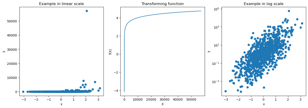
この関数では、引数として”log”などの文字列を与えると、Linear-Logで相関を持つデータを作り、それをLinear-LinearとLinear-Logで散布図をプロットします。散布図における変数変換の有用性を示すための関数です。
上記の関数を実行してみましょう。引数は”log”とします。以下を実行してみてください。
plot_example_scale('log')結果、以下の図が表示されます。
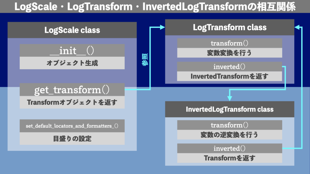
以上のように、Scale、Transform、InvertedTransformの相互関係(図3)を知っていると、Matplotlibを使って作図をするときにできることの幅が増えます。
Result | Pythonのサンプルコード
今回のPythonコードの実装例を掲載します(Jupyter Notebook)。参考にどうぞ!
Conclusion | まとめ
最後までご覧頂きありがとうございます!
Pythonの作図ライブラリMatplotlibに用意されたLogスケールに関係するClassを紹介しました!
Matplotlibでは、LogScale、LogTransform、InvertedLogTransformの相互関係を頭に入れたうえで、Log変換やLogの逆変換を扱えるようになると、Matplotlibを使った作図でできることの幅が広がります!ぜひ今回の記事を参考にしてみてください!
以上「Matplotlib | LogScale classとLog変換(Python軸スケール4)」でした!
またお会いしましょう!Ciao!
References | 参考
参考に本シリーズの記事と外部リンクをまとめます。
本シリーズの記事
- 第1回: Matplotlib | Python作図での軸のスケール設定の必要性(Python軸スケール 1. 知識編)
- 第2回: Matplotlib | 予め用意された7種類のスケール(Python軸スケール2)
- 第3回: Matplotlib | Scale Classの概要(Python軸スケール3)
- 第4回: 本記事
外部リンク
- matplotlib.scaleのドキュメント: https://matplotlib.org/stable/api/scale_api.html
- matplotlib.scaleのソースコード: https://github.com/matplotlib/matplotlib/blob/v3.10.1/lib/matplotlib/scale.py
コメント